Creating AlexNet on Tensorflow from Scratch. Part 2: Creating AlexNet
This is part 2 of a series where I’m going to go through creating AlexNet and training it on CIFAR-10 data, from scratch. This portion will talk exclusively about creating AlexNet based on the paper.
AlexNet

AlexNet assumes the input image is of size 224 x 224 x 3, where the 3 represents the RGB channel of a colour image. Since we are going to do this in batches (mentioned in Part 1), we’ll create a 4 dimension placeholder for the input image.
First Convolution Layer
“The first convolutional layer filters the 224×224×3 input image with 96 kernels of size 11×11×3 with a stride of 4 pixels.”[1]
From section 3.1 of the paper, it’s noted that AlexNet also applies ReLU nonlinearity after the conv layer.
The 3rd input parameter into the conv2d function is a list of [1, 4, 4, 1]. It has been described in the Tensorflow documentation for conv2d that “For the most common case of the same horizontal and vertices strides, strides = [1, stride, stride, 1].” In essence, it means that the horizontal and vertical strides are 4.
Note that the padding for conv2d is set to SAME. To understand what the padding does, you can read this insightful Quora answer. In short, if padding is set to VALID instead, the output shape will be different and it will affect the entire output structure of the model.
In section 3.3 of the paper, it mentions adding “Local Response Normalization” after ReLU. Luckily, that’s a function given by Tensorflow which we can just add after the first convolution layer. The result of that goes through max pooling.
Second Convolution Layer
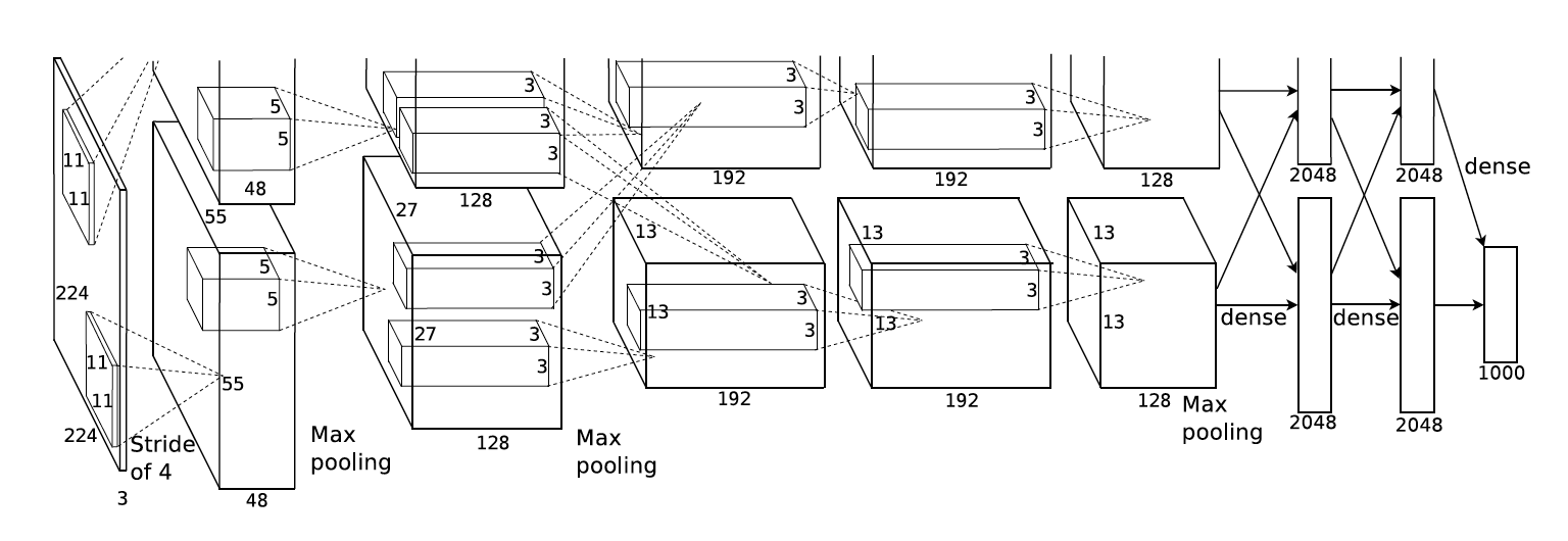
“The second convolutional layer takes as input the (response-normalized and pooled) output of the first convolutional layer and filters it with 256 kernels of size 5 × 5 × 48.”[1]
The process is similar to the first convolution layer. In fact, it is not uncommon to bundle the conv2d, bias, relu, lrn, and max_pool into one function. However, for the sake of this tutorial, I try to be more explicit in the code.
It is important to note that the input kernel for the second convolution layer is [5, 5, 96, 256]. The 5, 5 represents the 5 x 5 size of the kernel. However, instead of width48, width96 is used instead. From the architectural diagram of AlexNet, it shows that the first convolution layer is divided into two paths, each of width 48. Combining the two together creates a width of 96. Thus, the second convolution layer continues this path and this can be seen in [5, 5, 96, 256]. In essence, the convolution layer shape for each layer is [kernel_size, kernel_size, previous layer width, this layer width].
Third Convolution Layer
“The third, fourth, and fifth convolutional layers are connected to one another without any intervening pooling or normalization layers. The third convolution layer has 384 kernels of size 3 × 3 × 256 connected to the (normalized, pooled) outputs of the second convolutional layer”[1]
The addition of the third layer is very similar to the first two, as far as ReLU. This third layer doesn’t include lrn or max_pool.
Fourth and Fifth Convolution Layer
The fourth and fifth convolution layer is same as the third, except for some differences in the weights.
Both Fully Connected Layers
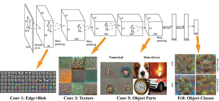
Each of the ConvNet described above extracts more and more complicated features from the images. The result of the final convolution layer is the most complex features extracted from AlexNet. An example of this is shown in the image below.

The result of this complex features now need to be classified, and this is achieved by two fully connected layers.
First Fully Connected Layer
The variable fc_size is set to 256, as that corresponds to the output of the last ConvNet layer. Before going through the fully connected layer, the result of the ConvNet is flattened to be a 1-D array using tf.layers.flatten. Once the data is flattened, it becomes a simple f(Wx + b) fully connected layer.
Second Fully Connected Layer
The second fully connected layer is like the first. There’s really nothing interesting to describe.
Output Layer
The final layer outputs based on n_classes, which is set at the beginning of the file. The variable out is the final output layer of AlexNet.
Sources
[1] Krizhevsky, Alex, Ilya Sutskever, and Geoffrey E. Hinton. “Imagenet classification with deep convolutional neural networks.” In Advances in neural information processing systems, pp. 1097–1105. 2012.
[2] Jeffries, Daniel. “Learning AI If You Suck at Math — P5 — Deep Learning and Convolutional Neural Nets in Plain…” Hacker Noon. February 27, 2017. Accessed August 06, 2018. https://hackernoon.com/learning-ai-if-you-suck-at-math-p5-deep-learning-and-convolutional-neural-nets-in-plain-english-cda79679bbe3.
